
Example: Use Worksheets with the What's New in Workday Report
This example illustrates how to use Worksheets with the
What's New in Workday
report. To do so, you want to create a workbook that includes:
- Live data.
- Note columns for each analyst and their assessments.
- Data validations.
- Formula columns that extract a list of features that affect your training materials.
- Adoption items.
You lead a team of 3 to manage the implementation of a Workday feature release. With each release, you and your team assess the
What's New in Workday
report to determine which features you:
- Must implement because they're automatically available.
- Can ignore.
- Want to consider for future adoption and the setup effort needed.
- Need to research to determine what changes to make to your employee training manual.
- Want to create adoption items for.
The steps use GMS tenant names Logan McNeil (you), Betty Liu, Steve Morgan, and Teresa Serrano. Substitute your team names for these names in your tenant.
Configure Worksheets and Drive, and give access to the feature planning analysts.
Security for you (not needed for the other users):
- Custom/Standard Report Copydomain in the Tenant Non-Configurable functional area.
- Set Up: Tenant Setup - Generaldomain in the System functional area.
- Copy a standard report to create a custom report.
- Access theCopy Standard Report to Custom Reporttask.
- SelectWhat's New in Workdayfrom theStandard Report Nameprompt.
- ClickOK.
- EnterRelease Planning with WN Report and Worksheetson theNamefield.
- ClickOK. (An alert displays on the page; you can ignore it.)
- On theColumnstab, click+to add a new column.
- SelectWorkday IDfrom theFieldprompt.
- On theAdvancedtab, select these check boxes:
- Enable As Web Service
- Enable for Worksheets
- ClickOK.
- Create a new workbook in Drive:
- SelectDrivein the Workday main menu.
- Select .
- UseWorkday [Release #] Release Planningas the name.
- ClickCreate.
- In the workbook, add live data using the report you created:
- ClickAdd Live Data.
- In theSelect Reportdialog, select theRelease Planning with WN Report and Worksheetsreport.
- ClickNext.
- In theSelect Prompt Valuesdialog, select:OptionDescriptionEnabled Functional AreasSelect the check boxWorkday Releases[Next release]
- ClickNext.
- In theSelect Columnsdialog:
- ClickSelect Allto add all of the report columns to the workbook.
- ClickAdd Note Column2 times to add 2 note columns.
- In theNotes Keyfield, selectWorkday ID.
- ClickNext.
- In the Select Options dialog, selectEnable Multi-Instance Valuesso that all enabled functional areas display in the workbook.
- ClickAdd. The Workday report runs and inserts the data into the workbook.
- Rename the Sheet1 tab and note column headings:
- On the Sheet1 tab, click the arrow on the right side of the tab and then clickRename.
- Rename the sheet asFeature Data.
- ClickOK.
- Double-click in each of the note column headings to rename them:From...To...Note1AnalystNote2Assessment
- Set up data validation values so you can create drop-down lists for assigning analysts to items, and for selecting an assessment result:
- Click+at the bottom left of the workbook to create a new sheet. Worksheets names the sheet Sheet1.
- On the Sheet1 tab, click the arrow on the right side of the tab and then clickRename.
- Rename the sheet asData Validation Values.
- ClickOK.
- Enter these values:AB1BettyImplement2SteveInvestigate3TeresaNo action
- In the Feature Data sheet, select the first cell in theAnalystcolumn.
- Click in the cell below the heading and go to .
- Enter these values:FieldValueCell Range to ValidateEnter a range that includes the entire column. Example:N:N.List of Values from FormulaEnter='Data Validation Values'!A:A.
- ClickOK.
- In theAssessmentcolumn, click in the cell below the heading and go to .
- InCell Range to Validate, edit the range to include the entire column. Example: Change the value fromO2:O2toO:O.
- InList of Values from Formula, enter='Data Validation Values'!B:B.
- ClickOK.
- In theAnalystcolumn, click in each cell and select an analyst from the drop-down list. (We recommend placing values in at least 20 of the cells, so that later steps in the example will display data.)
- Share the workbook with your analysts, giving Can Edit access:
- Click theShareicon at the top right of the workbook.
- In theShare with Individualssection, enter:
- Betty Liu
- Steve Morgan
- Teresa Serrano
- Type this comment in the message area:Analysts, please select an assessment value in each of the workbook rows assigned to you.
- ClickShare. The analysts receive a notification in their Inbox that contains a link to the workbook.
- The analysts can open the shared workbook, study the What's New Items assigned to them, and select a value in theAssessmentcolumn for each item. We recommend placing values in at least 20 of the cells, so that later steps in the example will display data.
- In a new sheet, extract information about What's New items that you're implementing, and that affect your training materials. Your education team can use this information to update their employee training materials:
- Click+at the bottom left of the workbook to create a new sheet.
- Name the sheetTrainingUpdates.
- Paste this formula into cell A1 of the sheet, replacing the final argument A1:O200 with the range of data in the Feature Data sheet:=SELECT("SELECT `Feature`, `What's New Item`,`Functional Area(s)`, `Feature Description` from ? WHERE `Training & Testing Impact` = 'This feature may require additional testing and may impact your training materials.' AND `Assessment` = 'Implement'",FeatureData!A1:O200)
- Press Ctrl+Alt+Enter (Windows) or Command+Option+Enter (Mac) to submit the formula.
- Add adoption items to your adoption dashboard:
- Go to theFeature Datasheet.
- In theWhat's New Itemcolumn, hover the cursor over an item until you see a link.
- Move the cursor to the far right of the link and click the outward arrow icon; this opens the What's New Item in a new browser tab.
- From the related actions menu of theView What's New Item, select . TheCreate Adoption Itemtask page displays, with fields from the workbook filled in automatically.
- Fill in any additional fields for the adoption item that you want.
- ClickOK.
- ClickDone.
- Repeat this step for other What's New items.
- Refresh the live data so that the newly added adoption items display in the workbook:
- In the live data panel, clickRefresh Now.(If you previously closed the panel to see more of the workbook data, you can display it again from .)
- ClickConfirm. The Workday report runs, and the workbook displays any new data; the adoption items you added display in the Adoption Item(s) column.
- Create a pivot table to see a summary of the analyst data:
- In theFeature Datasheet, select .
- In theCreate Pivot Tabledialog, leave the fields as is and clickCreate.A basic pivot table displays in a new Sheet1 and the Pivot Table panel displays.
- In the Pivot Table panel:
- FromAvailable Fields, findAnalystand drag it to theColumnsarea.
- FromAvailable Fields, findAssessmentand drag it to theRowsarea.
- ClickUpdate. The table updates to display a summary that looks similar to this image:
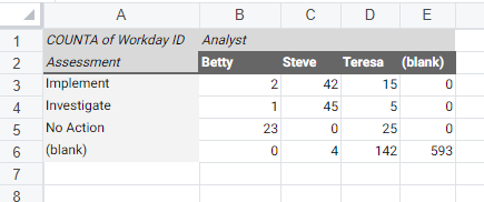
Optionally, you can create a formula column in the workbook to create working Community Post links in the live data area so that the links open the associated What's New posts instead of an instance page. (Worksheets doesn't support opening external links or attachments from a workbook.) To do this:
- In the workbook, create a formula column to the right of the Community Post column. Right-click theCommunity Postheader and select .
- ClickConfirmto do the live data refresh and create the formula column.
- Double-click theFormula1header and rename the header toCommunity Post (Corrected).
- In the first cell of the formula column, type the formula=IFERROR(HYPERLINK(F1),"None"), replacing theFcolumn identifier with the Community Post column letter in your live data.
- PressEnterto submit the formula. The IFERROR function causes cells without a Community Post link to display the textNoneand the HYPERLINK function takes the content of the non-working cell and creates a working link.
Refresh the live data at any time to bring in any corrected or newly added What's New items.
Create charts to track progress of analysis.
Share with others outside the team, giving them comment or view access, so they can see the assessments but can't edit the data.