Concept: Conditional Formatting in Workbooks

Conditional formatting enables you to apply cell formatting selectively and automatically, based on cell content. Conditional formatting is an easy way to quickly identify erroneous cell entries, cells of a particular type, or cells within a range of values. You can use a format (such as a gradient of a red background color) to make particular cells easy to identify. Sometimes conditional formatting is a better way to visualize your data than a chart.

You can apply formatting rules to standard data, unconstrained formula data, live data, and pivot tables.

You can assign single color or color scale (gradient) formatting rules based on formulas, or on preset conditions. Here are a few examples of pre-set conditions:

Greater than or equal to

Less than or equal to

Is equal to

Has errors

Text contains

Text begins with

Date

Above or below average

Cell is blank

To view the existing conditional formatting rules for a range of cells, select the range and then select

View

Panels

Conditional Formatting

. To display all conditional formatting rules for a sheet, select the top left cell in the workbook data area.

Worksheets doesn't support adding conditional formatting rules for data bars or icon sets. If you upload an Excel workbook containing data bars or icon sets, they aren't preserved in the Worksheets workbook.

Adding a Conditional Formatting Rule

To apply a conditional formatting rule to a cell or range:

Select the cell or range, then navigate to Formatting > Conditional Formatting
. The Conditional Formatting panel opens and the Apply to Range
field contains the range you selected.

In the Formatting Style drop-down menu, select Classic
for a single color rule or
Color Scale
for a color gradient rule.

Classic	Select the type of rule, the value to base the rule on, and the formatting for the cell or range if the rule is true.
Color Scale	Select the Minimum, Midpoint, and Maximum value type. If applicable for that value type, type the associated value to the right. Then select a color to associate with that value type. The Formatting example shows a preview of the condition rule's appearance.

(Optional) Select the Stop if true
check box if you have more than one rule and you want to stop processing the rules that are lower in the list when the first "true" condition is achieved.

Click Apply
.

(Optional) If you have more than one rule for the same range of data, you can drag rules in the Conditional Formatting panel to change their priority, or click the gear icon and then click Move Up
or Move Down
.

Considerations for Using Conditional Formatting

Keep these tips in mind when using conditional formatting:

If you apply a classic rule to your data, Worksheets sets the conditions correctly for either numeric or string values in the cells. If you use a color scale in your rule, the cell values must be numbers.

Avoid using the rule Greater than 1
in a full-column/row rule, because this rule can cause the header row's formatting to change.

If you insert rows or columns within a range that already contains conditional formatting, the newly inserted cells get the same conditional formatting.

When you press Delete to delete the contents of a cell, you don't delete any existing conditional formatting. To remove all conditional formats and all other cell formatting, select the cell and then choose Edit > Clear > All
.

You can associate both classic (single color) rules and color scale (gradient) rules to the same set of cells, but we don't recommend it because you might see unexpected results.

When you have multiple rules in a priority list, Worksheets doesn't apply the same formatting (such as background colors) again in subsequent rules. For example, if you have a rule to apply formatting when a value is less than 6, then in a later rule you apply formatting when a value is less than 4, Worksheets won't apply the same formatting with that later rule. If you do want that behavior, you need to place the "less than 4" rule higher in the rule list than the "less than 6" rule.

When you download a workbook, Worksheets doesn't preserve these conditional formatting rule types:

Top 10

Unique values

Duplicate values

Contains (text)

Does not contain (text)

Ends with

Begins with

Contains blanks

Does not contain blanks

Contains errors

Does not contain errors

Time period

Above average

Examples of Conditional Formatting

This workbook sheet has 3 conditional formatting rules. You can experiment using this workbook and the example rules below to see similar results.

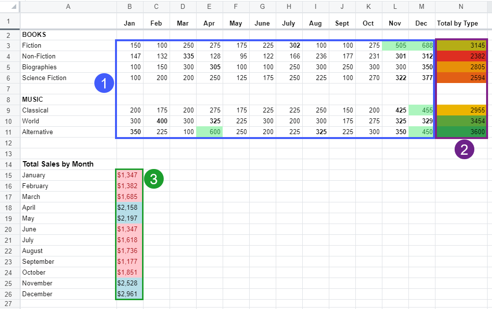
1: Two Rules, including a Stop If True setting

The first rule changes the font color and cell background color for the top 5 values in the range.

Because of the Stop if true
setting, after identifying the top 5 values, Worksheets doesn't process the second (bold) rule.

The second rule formats all values greater than 300 in Bold
. The top 5 values, even though they're over 300, are not bold because we stopped processing the rules as soon as we identified the 5 values.

2: Color Scale Rule for lowest to highest values

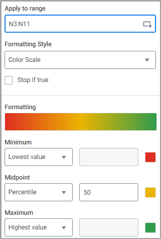
The lowest to highest values in the range are shaded from red, through yellow, to green, with a percentile to indicate the middle of the range.

3: Two classic rules for pink and blue formatting

Greater than and less than classic rules

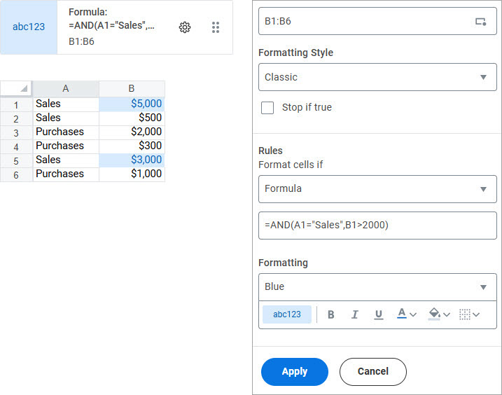
Example of Conditional Formatting Using a Formula

The Formula
option in

Rules

can be used when the conditional formatting needs to consider multiple conditions. This example has a conditional formatting rule that uses the AND formula with 2 conditional statements. The formula identifies all rows with Sales
in the first column and then changes the cell background color for the value in the second column to blue if that value is greater than $2,000.