
Concept: Editing Workbooks
These notes describe how to use workbook features in Worksheets that differ from other spreadsheet applications. For more details, see the Worksheets User Guide, which you can access from the Worksheets user interface ().
Workbook Editing
Action | Notes |
|---|---|
Use full-screen mode | In full-screen mode, Workday hides the header to display the maximum possible number of workbook rows. Select . Workday doesn't support full-screen mode in the Safari browser. |
Add Workday report data into a workbook | We use the term live data for Workday data that you add to a workbook. Select the cell where you want to insert the data and click Add Live Data . The Data Wizard opens and helps you find the report and add the data. You can select whether to add the data as:
You can add data from more than 1 Workday report into a single workbook. We recommend using a new sheet for each set of live data. Worksheets doesn't support using the Do Not Prompt at Runtime prompt option in a report definition. |
Refresh all live data in a workbook from 1 or more reports | You must have permission to edit the workbook and to refresh live data. When you do a refresh, Worksheets also recalculates formulas affected by changed workbook data.
You can refresh all live data areas in the workbook and recalculate:
When you recalculate and refresh the live data in a workbook, Worksheets updates all data, including data in a protected range. You can't prevent Worksheets from refreshing and recalculating workbook content. Example: When you update an entry area in Workday Projects, or Workday runs a scheduled live data refresh, Worksheets updates any necessary data even if you protected the entry area or live data range. |
Refresh live data in a single range from the associated Workday report | In the workbook, select a cell that includes live data. In the live data panel, click either:
|
Edit workbook live data areas (add, remove, or reorder report columns) | Click the Edit link in the Columns section of the live data panel. Alternatively, you can click any of the Edit links in the panel, or the Edit Live Data button at the bottom of the panel.)Live data column editing applies only to live data from advanced reports. Worksheets doesn't update data references in formulas when you edit live data columns; you need to manually update formulas that refer to any live data area that you edit. |
Schedule live data refreshes | (Workbook owner only) In the workbook, select . For workbooks already on a schedule, select . You can also select this option to edit or delete an existing schedule. At the scheduled time, Workday automatically:
For any prompts in the Data Wizard where you selected the Use Report Default option, Worksheets uses the default values from the report definition when refreshing the data; otherwise, Worksheets uses the current prompt values displayed in the live data panel. You can create 1 schedule per workbook. When Worksheets runs a scheduled refresh, the updated data is available to users with shared access to the workbook. If workbook ownership changes, the schedule stops running; the new owner must create a new schedule. If the Workday report associated with the live data refresh times out 3 times consecutively, Worksheets automatically cancels the refresh and pauses the schedule. If Worksheets pauses a schedule, the workbook owner receives a Workday notification that includes a link to the affected workbook. After you fix the problem that caused the report failure, you need to manually resume the schedule by clicking Resume in the live data panel in the workbook.Worksheets doesn't preserve schedules when you refresh a tenant from a tenant with a different name. You need to create new schedules for the workbooks in the new tenant. Example: You refresh the company_name_preview tenant from the company_name tenant.If a worker sets up a scheduled live data refresh and then leaves the company (and is in a terminated state), the scheduled refresh returns an error in the workbook because Workday can't run the associated report. |
Undo or redo your changes | To undo a workbook change, select . To redo a workbook change, select . Worksheets tracks your most recent 15 changes that you can undo. When you select an action that you can't undo, Worksheets displays a confirmation message. If you continue with the action, Worksheets resets the record of your changes. You can't undo earlier changes, unless you previously created a named version. Keep in mind that when another person edits the workbook, they might perform an action that resets change tracking and prevents you from undoing a change. We recommend creating a workbook version () before doing any of these actions, which Worksheets can't undo:
You can't undo changes to workbook comments, and reverting to a previous version doesn't restore comment changes. |
Define or edit conditional formatting rules | Select the cell or range, then navigate to . To view the existing conditional formatting rules for a range of cells, select the range and then select . To display all conditional formatting rules for a sheet, select the top left cell in the workbook data area. |
Insert subtotals and a grand total | Worksheets can automatically insert subtotals for sets of related data in your workbook, and calculate a grand total. Select a single cell to indicate the column of data you want to add a subtotal for. Then select and fill in the fields. You can't add subtotals in entry areas. |
Group (outline) data | Select the rows or columns that you want to group, right-click, and then select Group . After grouping, you can select a group, right-click, and Ungroup a single group, or select Ungroup All to remove associated groupings. |
Define data validation rules | You can define rules that determine what data can go into a set of cells in your workbook. Example: You want to make sure that users select a geographic region from a list of valid regions, which your workbook stores in another column.
|
Rename or copy a workbook sheet | To rename the sheet or to do other sheet actions, click the arrow on the sheet tab. Sheet names can be up to 31 characters long. We recommend using names of 27 characters or less. When you copy a sheet, Worksheets uses 4 characters to add a space and a numerical increment in parentheses to the sheet name. Example: When you copy the sheet named My Sheet , Worksheets names the copy My Sheet (2) . When you copy a sheet, Worksheets doesn't preserve protected ranges in the new sheet. |
Open instance details in a new browser tab | When a workbook includes instance details, you can open the link to view them. To open the instance page in a new browser tab, select the icon in the instance link or use Ctrl+Click (Windows) or Command+Click (Mac). |
Collaborate |
|
Define a name | Select the cell or range, right-click, and then select Define Name .Defined names must be unique per workbook, and can be between 4 and 255 characters long. When selecting a defined name in the formula drop-down menu using the keyboard, use Tab (not Enter) to select it. |
Protect ranges | (Workbook owners only) To prevent other users from editing a cell or range, select the cell or range and then select . To protect a sheet, click the sheet menu (the down arrow on the sheet tab) and then select Protect Sheet .When you recalculate or refresh the live data in a workbook, Worksheets updates data even if that data is in a protected range. |
Find content in a workbook sheet | To find values in a workbook sheet, select or press Ctrl+F (on Windows) or Cmd+F (on Mac) to open the Find in Sheet panel. You can search for values, but not formulas.When you search in a workbook, Worksheets displays results that contain the characters you type, in the order you specify. The default search is a wild card search, with an implied asterisk character (*) at the beginning and end of the string you specify. For advanced searches, start your query statement with the ^ character. |
Break a line in a workbook cell | Double-click the cell in which you want to insert a line break. Click the location inside the selected cell where you want to break the line. Press Alt+Enter (Windows) or Option+Enter (Mac). If you use the workbook formula editor, it removes line breaks, so you need to add the breaks again. |
Delete workbook sheets | Click the sheet menu (the triangle icon on the sheet tab) and then select Delete .Worksheets can't undo deleting a sheet. |
Create pivot tables | Select the range to include in the pivot table and select . Pivot tables containing live data rely on the report column names from the Workday report. If you change a report column name in the report, and that data is used as a field in a pivot table, you need to replace the pivot table field associated with the original name with the field that's based on the new report column name. |
Refer to data in other workbooks | To add external (cross-workbook) references, you must have edit permission for the consumer and view permission or higher for the producer workbook. A workbook that refers to (brings in) data from another workbook is a consumer workbook. A workbook containing data that's being referred to in another workbook is a producer workbook. A workbook can be both a consumer and a producer.From a producer workbook, you can copy a reference, then paste it into a consumer workbook:
From a consumer workbook, you can copy the Workday ID of a producer workbook, then add the defined name, or sheet name and cell/range reference manually:
Consumer workbooks display an External References icon on the workbook toolbar. The icon turns green if data in the producer workbook was changed. You can click the icon to update the data in the consumer workbook. The update that occurs as a result of the action is the same as Recalculate All. Once the producer workbook's data changes occur, there might be a delay of up to 2 minutes before the consumer workbook External References icon turns green. |
Merge 2 workbooks | You can add the sheets from another workbook into the open workbook if you're the owner or you have edit permission. Open the workbook that you want to contain all the content from both workbooks, then select . When merging workbooks, Worksheets doesn't:
If updatable data, such as from an entry area, exists in the workbook you're selecting to merge content from, Worksheets copies the values from that area but no longer considers the data updatable. |
View quick statistics on a selected range | When you select a range of cells in a workbook, such as defined names, columns, or sheets, these formulas display to the right of the formula bar to provide quick reference statistics about your selection:
Based on the types of data in the selected cells, Worksheets shows the relevant functions in the drop-down list. For SUM, AVERAGE, MIN, and MAX, Worksheets converts units in the same dimension (such as length) to determine the result. If all selected cells contain non-numeric data, then Worksheets displays only the COUNTA statistic. |
Create a workbook version | Workbook versions provide a checkpoint for a group of changes. Select , then type a version name in the Add Version to Workbook dialog.Workbook comments are independent of any versioning status: the user sees in the Collaborate panel all comments entered for the workbook, regardless of the version where the comment was added. Restoring to a previous version of the workbook doesn't undo or change the Collaborate panel data. |
Sort data, including advanced sorting of live data and contiguous columns | Select the columns or rows to sort, then select and then select a sort order or select Advanced Sort . You can sort live data areas and entry areas in a workbook. Optionally, your sort can include contiguous columns in the workbook that are outside the live data area or entry area. By default, if your workbook sheet contains live data and you select Advanced Sort on the menu, Worksheets selects only the live data area for the sort. If you want to include additional columns in the sort, highlight the entire range that you want to sort before selecting Advanced Sort .When you refresh live data in a workbook, Worksheets preserves the sort order that you set in the Order By option in the data wizard, but doesn't preserve standard sorting within the workbook (using ). |
Paste content into a workbook | You can use Ctrl+C and Ctrl+V to copy and paste content as values from 1 Worksheets workbook to another, or from a desktop spreadsheet application such as Excel. You can't use the workbook menu option to paste desktop application content into a workbook; Paste Special works only between workbooks that currently reside in Worksheets. Import (upload and convert) the desktop spreadsheet into Worksheets by selecting before pasting data from it that includes formulas into a Worksheets workbook. You can copy and paste up to 9 MB of content from 1 workbook to another. |
Freeze spreadsheet cells | Locate the freeze handles in the top left corner of the sheet. 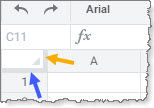 Drag a handle to freeze columns or rows. Alternatively, you can scroll until the desired column or row is in the first viewable position in the workbook, then freeze at that position by selecting . Worksheets freezes at the location of the first visible row in the spreadsheet, which might not be row 1. Similarly, selecting freezes at the position of the first visible column in the workbook. To unfreeze all columns and rows, select . |
Navigate within a range of cells | If you select a range of cells and then press Tab to move from cell to cell, the cursor stays inside the selected range. |
Insert a chart | Select the data to include in the chart, select , then select a destination cell for the chart. The chart starts at the selected cell and displays in an area of merged cells that's approximately 10 rows in height and 4 columns in width. If you include date information in the chart, make sure that you use standard date/time formats; otherwise, Worksheets doesn't recognize the information as dates. Keep in mind that if you use a pivot table as the source data for a chart, and later you change the rows, columns, or values to include in the pivot, you need to make sure your chart still displays correctly. |
Auto-fill a formula or value into all cells in a column | These steps provide a keyboard alternative to using drag-fill:
|
Change the font | Worksheets supports a variety of widely available fonts. The default workbook font is Roboto. Worksheets doesn't support the Calibri font. |
Rebuild a corrupted workbook | If a problem, such as a system error or an interrupted process, causes a workbook to be corrupted, you can return the workbook to a working state using a keyboard shortcut:
|
Formulas
Task | Notes |
|---|---|
View reference information for all available formulas | Click the Function icon (fx) to open the Functions Library panel. |
Enter a formula | Use one of these methods:
To treat the data in a cell as text instead of a formula, type a ' (single quote character) before the = character. Worksheets treats everything after the ' as plain text. The ' character doesn't display in the cell, but it displays in the formula bar. |
Submit a formula from the formula bar or the cell containing the formula | If you expect the formula to return a single value (it's a scalar formula), press Enter to run the formula. If you expect the formula to return multiple values (it's an unconstrained array formula), use the Ctrl+Alt+Enter (Windows) or Command+Option+Enter (Mac) keyboard shortcut. |
Submit a formula from the formula editor | Click Save & Close . When you open the formula editor for a formula, the editor detects if the formula is a standard scalar (single value, nonarray) formula or unconstrained array formula, and submits it appropriately. Worksheets doesn't support using the formula editor for constrained array formulas. |
Enter numbers into a formula | You can enter numbers in several formats, such as:
The cell might not display the number exactly as you typed it, depending on the current cell formatting rules and other factors, but Worksheets preserves the value. To make Worksheets handle the format of the cell as text, type a ' (single quote character) before the = character; Worksheets treats everything after the ' as plain text. The ' character doesn't display in the cell but it displays in the formula bar. Example: You can enter dates and preserve the formatting you typed, instead of displaying it in a format such as DD/MM/YYYY. |
Circular References
In almost all cases, a circular reference indicates an error that you must correct.
We strongly recommend not enabling iterative calculations, particularly in workbooks that contain live data; doing so obscures data errors that can lead to poor performance and unexpected behavior.
A red icon indicates that Worksheets didn't finish calculating; the workbook is in a state where some formulas didn't fully run and are showing stale values. You can hover the cursor over the icon to see a tooltip with information about the problem. There are two common causes for a workbook to prematurely stop calculating: either the calculation limit was reached, or one or more circular references exist in the workbook. If the problem is caused by a circular reference, you can click the red icon to navigate to the cell location of the reference. If you have more than one circular reference, Worksheets navigates to the location of the first one.
In rare situations, you might want to enable circular references. Example: You have a basic cost of $1,000,000 for a project. A consultant earns a 5 percent fee based on the total project cost, which is $1,000,000 plus the consultant fee. Because the fee is part of the calculation, it's a circular reference in the spreadsheet, so you need to enable iterative calculation to occur.
A | B | C |
|---|---|---|
Basic Cost | $1,000,000.00 | |
Consultant Fee | =B3*C2 | 5% |
Total Cost | =SUM(B1:B2) |
To enable the calculation of circular references in a workbook, select , select
Enable Iterative Calculation
, and add values for:
- Maximum iterations: 100 or fewer.
- Maximum change: Enter a maximum change value. The default is 0.001. Worksheets does the circular calculation for the number of iterations that you specified, or until the result changes by less than this value.
If you open a workbook containing circular references, and your recalculation setting is
Manual
, a message displays; select to update the data.